Here we will explain you how we make our comparisons with distillation test
data with mass transfer coefficient (MTC) correlations in ChemSep.
We'll use data on Sulzer BX packing as an example. It was published in an
article in Chemical Engineering Progress of January 1998 (p.60),
by Mike Lockett. The data originated from the Fractionation Research Institute
FRI. In the article Lockett also compared the
data with the mass transfer model of Bravo, Rocha, and Fair (Hydrocarbon
Processing, January 1985, p. 91), which we abbreviate with BRF85.
Lockett's article features "measured" HETP's which are plotted as a function of
the packing F-factor, at four different pressures, in his figure 1. It is important
to note that these HETP's are not measured as such but they are computed by
simulating the distillation tests with an equilibrium stage simulator while matching
measured bottoms and tops compositions. To get a good match one stage is to be taken
to have a fractional stage efficiency (between 0 and 1). The HETP is then resulting
from the bed height divided by the number of stages in the simulation (of course,
excluding condenser and reboiler. If the vapor velocity in the bed changes it is
important to use the location with the highest flows for computing the F-factor.
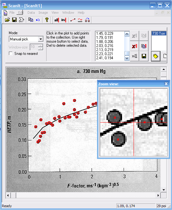
For the example here we will use a scan for Lockett's plot of HETP's for the
o/p-Xylene system at 1 atmosphere, Figure 1a.
We could read the values from this graph by hand but to get a little more precise
numbers we use the tool ScanIt to
obtain the datapoints. ScanIt lets you pick the origin and two axis end points of the
Figure to determine the scale of the scan. After this you can select each point with
the mouse and ScanIt will mark it and compute the x,y values of the original datapoint.
With the "Copy data" button we can copy the data to the clipboard. We open a Notepad
text editing window and paste the data in there. We also add some descriptions in this file:
.
We chose a naming that is a reference using an abbreviated journal name, followed
by the volume number, a small "p" for page, and then the page number. This usually
generates an unique name. When the journal does not use volume numbers but year and
month instead, we use those, with the month as three small letters. For conferences
we use an abreviated conference name, year, and a session number or a page number
of the proceedings.
The resulting text file can directly be plotted with ChemSep using the
"Plot data file" menu-item under Analysis. The plot can be made to ave the same
axii as it was originally published with as well as labels in the plot.
When multiple experimental data sets are shown in one graph it is better to
separate them into separate files and call them for example fig1a, fig1b, fig1c etc.
This will allow them to be used separately in model comparison studies as we will
see below. You can always combine them into one figure by adding another text file,
for example as "fig1", by appended the files into that file. Make sure you give each
set a different label and color/point-type so that they remain distinguable!
Our example will look like:
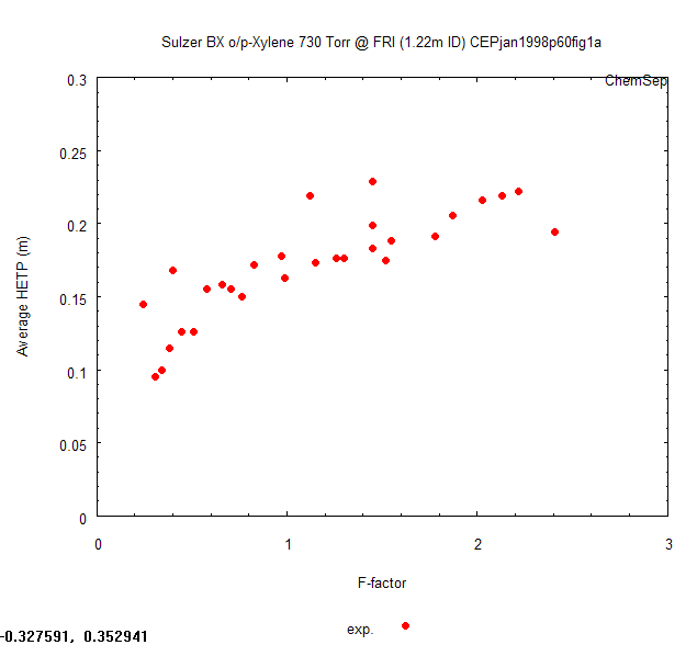
Showing the distillation test data with the "Plot data file".
How to Compare MTC predictions with Distillation Test Data
To make this comparison you need to setup a simulation of the distillation tests
in ChemSep for the system in question. We like to use the same filename as the
dataset and add to it the model name (abbreviation), for example for the BRF85 model
Structured/Sulzer/BX/cep1998janp60Fig1a_BRF85.sep.
The easiest way to get this done is by searching our online database for a simulation
(sep) file with the same distillation test mixture (and pressure) and adapt it for the
right packing, bed height, and MTC model.
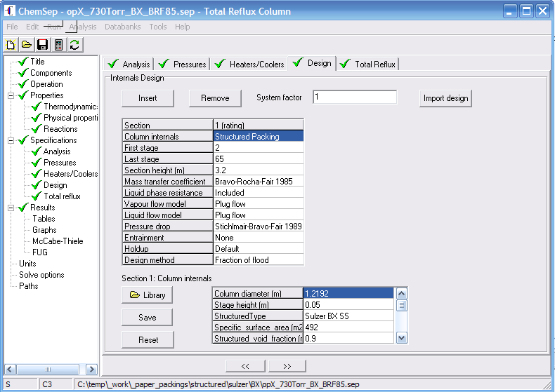
Setting up the o/p-xylene simulation with the BRF'85 MTC model.
When we have a converged simulation and verified it is correct we need to simulate it
at various flow rates. For this we use parametric study option (under "Analysis") in
ChemSep. We vary the reflux flow to the column to simulate the tests at different vapor
loadings. You might need to play a little with the liquid reflux rates to obtain the right
range for the test data. Note that we chose to plot the average HETP, by using AHETP1.
This computes an average HETP over the whole bed of section number 1. We plotted it as
function of the F-factor on stage 35, which resides in the middle of our bed.
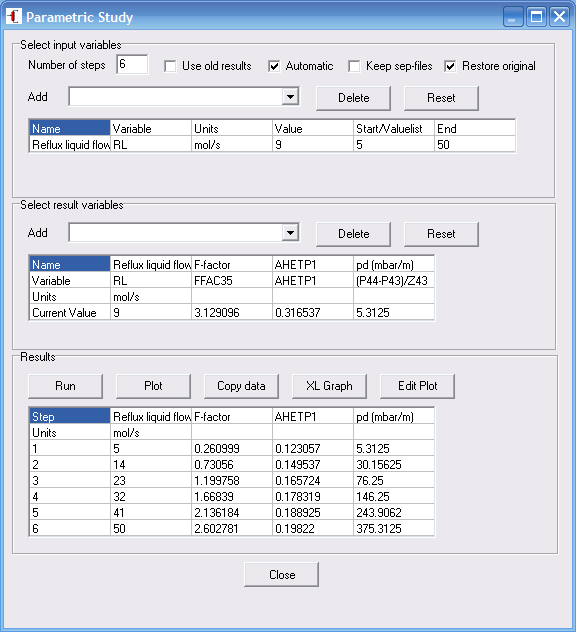
Using Parametetric Study to simulate the column at different vapor loadings
(and hence F factors) and calculating the average HETP.
Then plot the data points again with the "Plot data file" menu item and switch on the
"Graph settings". This will allow you to add a data-set wth the "Add set" button.
Here we plot the second and third column in the Parametric Study, by using the identifiers
PS2 and PS3, on axii x1 and y1 for the 6 points generated in the Parametric Study (adapt
this if you use a different number and indices for the variables).
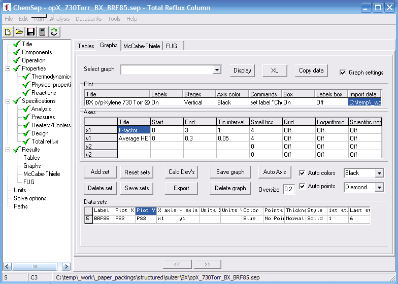
Use "graph settings" to add the BRF'85 prediction next to the experimental data.
When we now click the "Display" button we obtain the experimental HETP and the
model predicted HETP in one graph. We see that there is quite a good agreement with
Lockett's publicated model predictions for the BRF'85 model. Deviations stem from using
the average HETP, different physical properties and the use of a full nonequilibrium
model. It is important that we use a sufficient number of stages to integrate the
packed bed and the correct flow models are chosen in the simulation, of course.
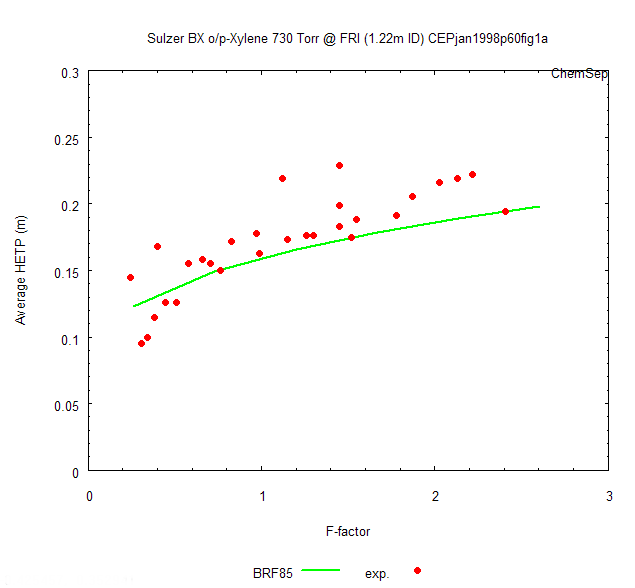
The BRF'85 prediction with the FRI experimental data for Sulzer BX packing with
o/p-Xyelene at 1 atm shows a good agreement.
To compare varous MTC models we need to be able to also compute the standard deviations
in this plot. It would also be nice if we can visualize the model deviations. We can!
Simply click the "Calc Dev's" button and these deviations will be computed for all data points.
Note that the range of the parametric study must be large enough for this to work. ChemSep uses
rational inter- and extra-polation to compute the model HETP's for each data point. The overall
standard deviation in HETP and relative HETP is also added as label to the graph. This is all
written to a new data file which includes the deviations as individual line pieces, and ChemSep
asks you to specify a new name for this file. Typicaly we append a digit for the text file, for
example: Structured/Sulzer/BX/cep1998janp60Fig1a1.txt.
When you inspect this file you see also that ChemSep appends a label with the deviation and
the relative error:
# string 0 0.3 s=0.024 r=0.143 b=+0.012
This allows you to further add other labels to the graph. The label may contain spaces but
special characters might not print properly.
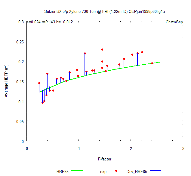
The BRF'85 model shows a relative standard deviation of 14 per cent or 24mm on an HETP
that increases from 120mm at low vapor loadings to 200mm at high vapor loadings. Note that
the bias is positive (+12mm), meaning that the BRF'85 model is 7 per cent optimistic in its
prediction of the HETP!
We are now ready to compare the results for different models and select the best MTC model
for this packing (and distillation system). We welcome anybody to contribute to our online
database of distillation tests. We try to cover all industrially relevant packings. Obviously,
this only works if the vendor makes its test data available or someone publishes measured
distillation tests on the packings.
This page is under construction. Submissions are welcome.
Copyright © 2008 ChemSep